Convolutions and Image Filtering

Abstract

All images can be represented as discrete approximations of functions and represented in the frequency domain. Images can be filtered through the use of convolutions in order to remove different frequency signals from an image. In this project I used filtering to blur, flatten, and blend images as well as create hybrid images which appear different from different viewing distances.

Introduction

From a somewhat nontrivial perspective images can be thought of as discrete samples of continuous multivariate functions where the function takes in an x, y coordinate of a pixel and returns the brightness of that pixel (or pixels in the case of colored images). This discrete sample of a function can be thought of a two dimensional discrete signal. From this perspective it becomes very natural to approach the problem of making systematic transformations to the image using convolutions. Convolutions allow us to make local transofrmations across entire images and have several nice mathematical properties which make them a well-fit candidate for image processing and filtering. In this project I show how these perspectives of images and the use of convolutions can be helpful for many different applications.

Edge Detection and Blurring

Edge detection in image processing is the process of automatically finding edges of objects in an image. Edges by definition are signficant local changes an image‘s intensity. The gradient of a function represents the direction and magnitude of local change and since images can be represented as functions we can use the gradient of the image to detect the intensity of local changes in an image. Note that we only have discrete samples of the underlying image function so we can‘t take the derivative directly and must instead take an approximation. In this case we can recognize that the partial derivative for each direction of the image can be approximated by subtracting the value of the previous pixel from the current pixel for each pixel in the image. Which can be represented as a convolution operation with the following kernels for the x and y partial derivatives respectively.

We can see the results of convolving these kernels (applying these filters) in the images below. We can see that by taking the norm of the partial derivatives in the x and y directions we get the gradient magnitude of the image which works as a primative edge detection operator for the image. If we binarize the gradient magnitude through some threshold value that we choose we can get a mask of just the edges.

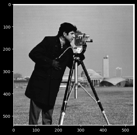
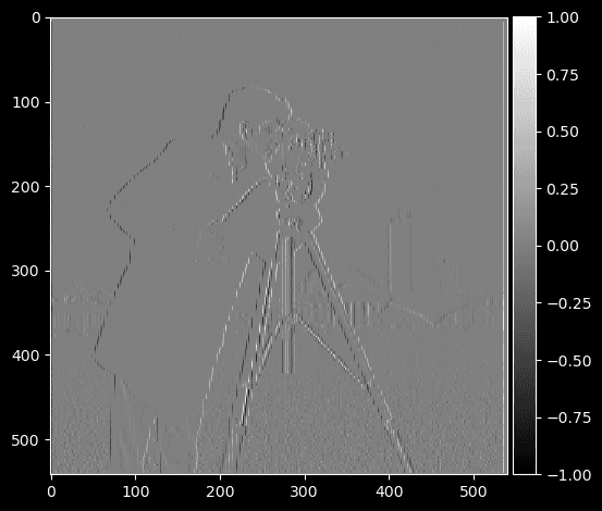
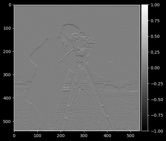
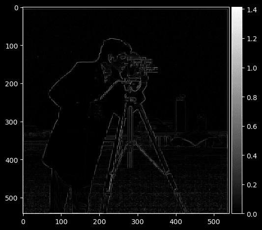
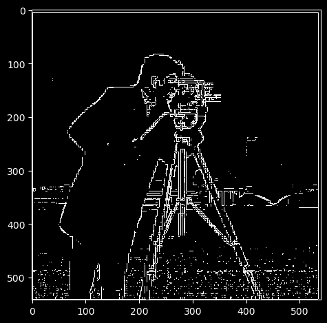
We can see however that our edge detection has some imperfections. In particular there are several artifacts in the image which are not edges that were captured. If we try to lower our threshold value to remove these artifacts we end up potentially losing actual edges. In order to fix this issue we can first blur our image before taking the gradient in order to average out artifacts with surrounding pixels thus improving out edge detection procedure. In order to blur our image we can use a low-pass filter which only lets through lower frequencies and removes high frequencies. We will use a 2D gaussian kernel and convolution to blur our image to avoid aliasing and get a smooth blur.

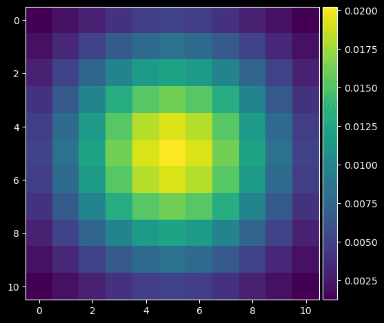
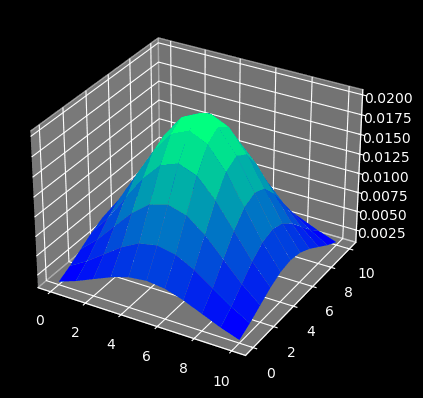
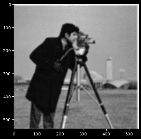
After blurring our image we can then take the gradient, like earlier, resulting in much cleaner edge detection with fewer artifacts. Due to the commutative property of convolutions we can also combine our partial derivative and gaussian kernels through convolution to create a deritive of a gaussian or DoG filter which when convolved with the original image gives the same result as first blurring then taking the gradient.

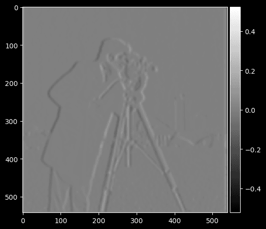
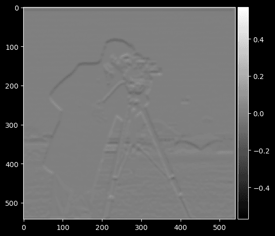
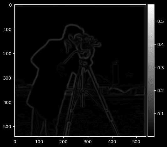
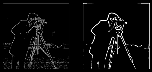
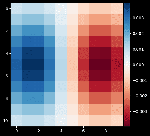
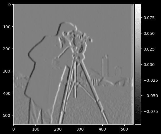
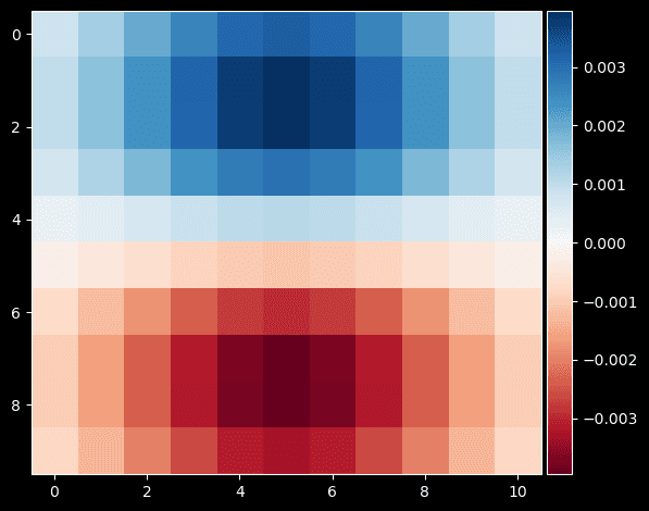
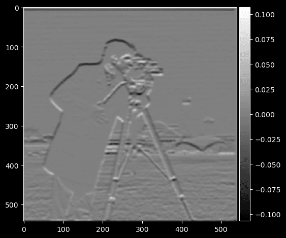
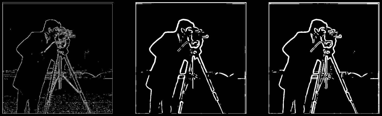
Image Sharpening

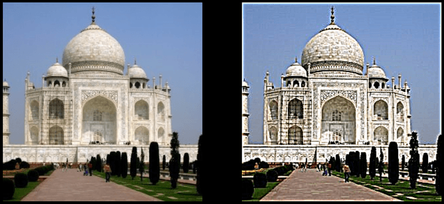
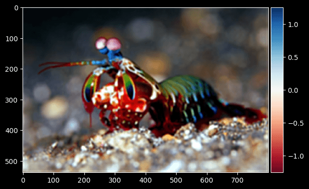
Image sharpening is the process of enhancing the high frequency details of an image. In order to accomplish this we can take a relaitvely simple approach stemming from image blurring. For image blurring we used a low-pass filter so it is only natural that for image sharpening we can use a high-pass filter which only lets through high frequency signals from and image. By simply subtracting the low-pass filtered image from the original image we can acomplish exactly this. In order to sharpen our image we can then multiply our high frequencies by some constant value and add them to our original image. Through a simple derivation and use of the Dirac delta function we can create a new filter known as the unsharp mask filter which can all be represented as the operation below.

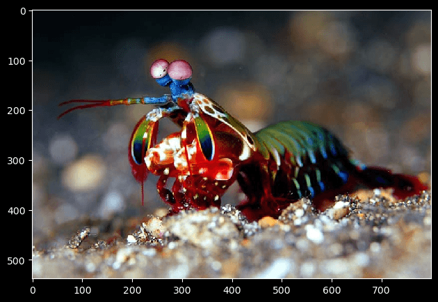
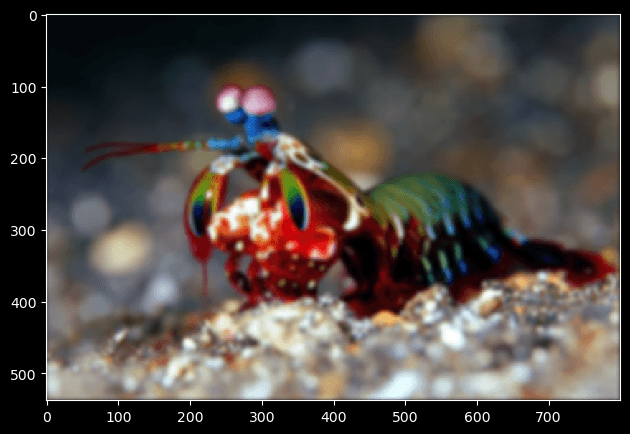
Through this procedure we get the following result pictured below. We can also see what happens if we first blur and already sharpened image then resharpen using our procedure as shown by the mantis shrimp images in the figure below.

Hybrid Images

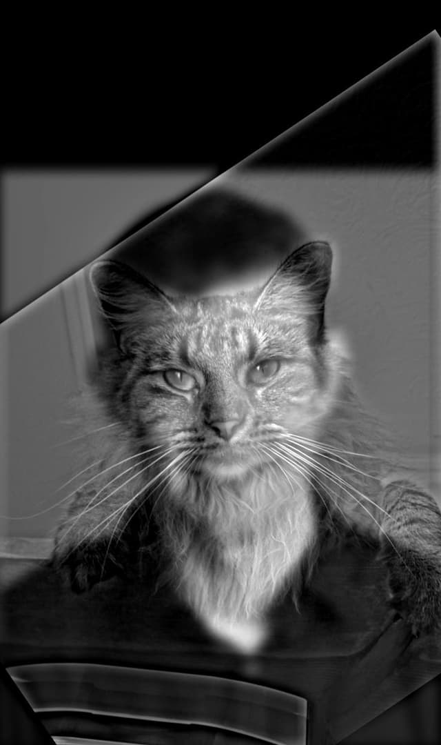
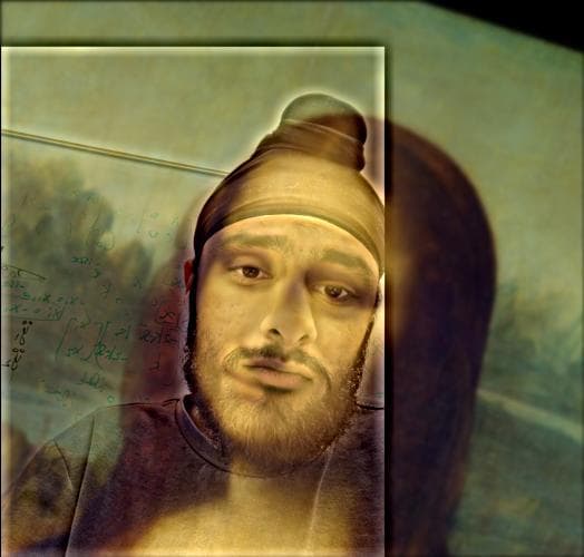
Now we will use our high-pass filters, low-pass filters and the approach described in the SIGGRAPH 2006 paper by Oliva, Torralba, and Schyns to create hybrid images. Hybrid images are static images that change in interpretation as a function of the viewing distance. The basic idea is that high frequency tends to dominate perception when it is available, but, at a distance, only the low frequency (smooth) part of the signal can be seen. By blending the high frequency portion of one image with the low-frequency portion of another, you get a hybrid image that leads to different interpretations at different distances.

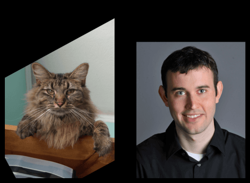
Our first hybrid image will be a combination of a man and his cat. Note that as a preprocessing step for all hybrid images we first align the images based on some manually selected points. We will add a low-pass filter of the man and a high-pass filter of the cat in order to yield our hybrid image. In this case we are using gray images, but we can get similar generalized results from RGB images.

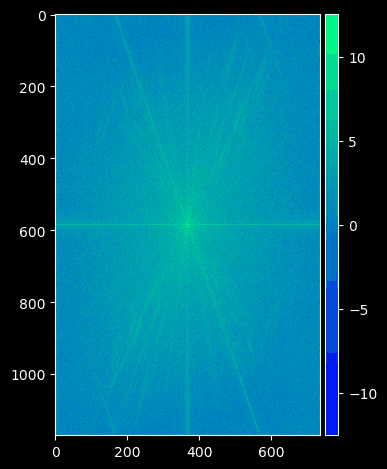
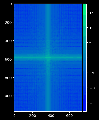
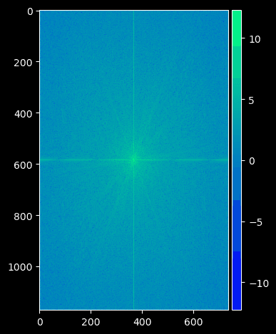
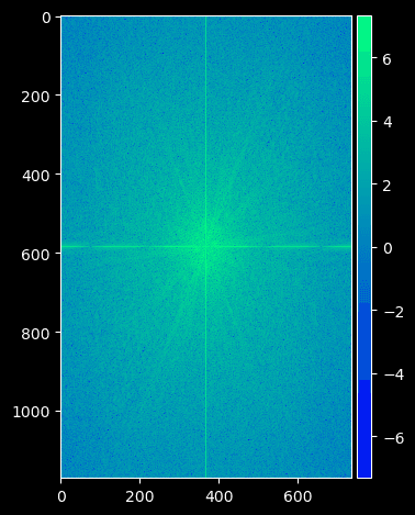
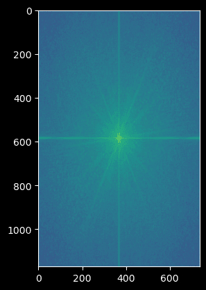
From a frequency domain perspective we can get a more geometric interpretation of filtering and hybrid images. By comparing the visualization of the amplitude versus frequency plots of the fourier transforms of each of the images and their respective filters we can see how each of the filters attenuates certain frequencies depneding on their respective filter. We can then see the resultant hybrid images fourier transform when we recombine the images.

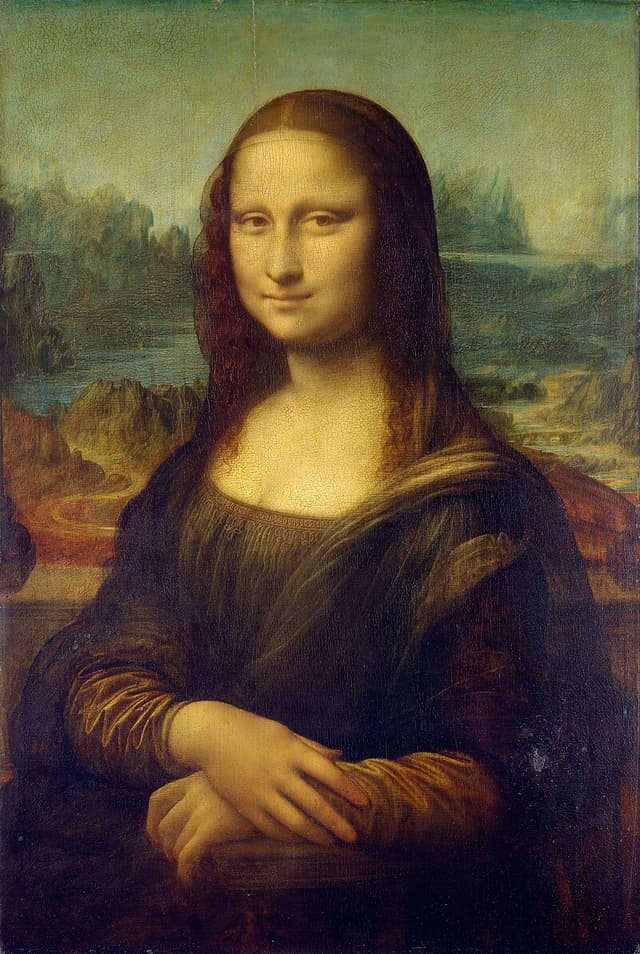
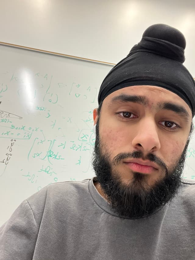
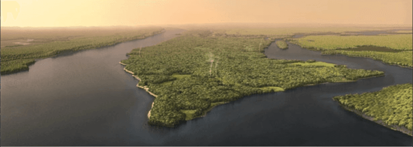
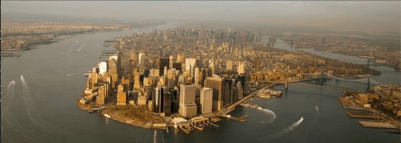
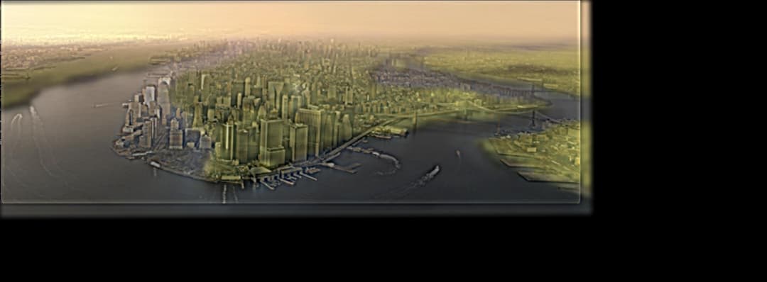
Below we are using hybrid images to superimpose my friend Amitoj Singh with the Mona Lisa and to superimpose New York City before and after its creation which both yield interesting results.

Blending Images

We will now use filters to blend two images seamlessly using a multi resolution blending as described in the 1983 paper by Burt and Adelson. An image spline is a smooth seam joining two image together by gently distorting them. Multiresolution blending computes a gentle seam between the two images seperately at each band of image frequencies, resulting in a much smoother seam. We‘ll approach this section in two steps: creating and visualizing the Gaussian and Laplacian stacks and blending together images with the help of the completed stacks, and exploring outcomes.

We will use both gaussian and laplacian stacks in or image blending algorithm. In order to create a gaussian we must iteravely convolve the same gaussian kernel over successive images. The end result will be a list or stack of images which progressively get blurrier. In order to create a laplacian stack we can simply take the nth level of the gaussian stack and subtract the n+1th level of the stack. This will progressively band-pass filter our image with the final level of the stack just being the final level of the gaussain stack.

We can now blend our images using the a modified version of the algorithm defined the aforementioned paper. We first create laplacian stacks for each of the images. We then get a mask which will define the boundary along which we want to blend our images. We take a gaussian stack of our mask and use it to smooth the transistion between images. For every level of the laplacian stacks we multiply by the corresponding level of the mask gaussian stack for the first image, and 1 - the corresponding level of the mask gaussian stack for the second image. We then add these two products to get the nth level of the combined stack. We can get our final result by adding all levels of the combined stack. We will first blend and apple and an orange along their veritical midpoint to create the oraple.

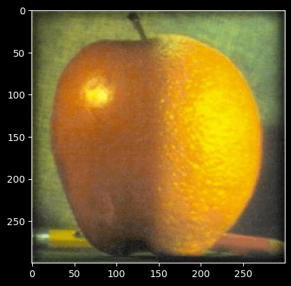
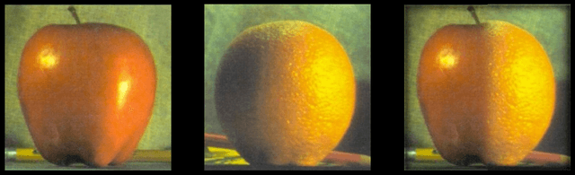
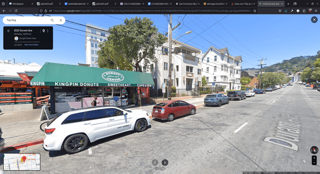
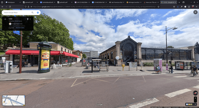
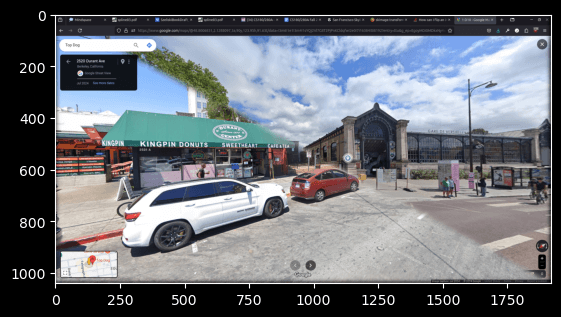
If we use a different mask we can get different results. Below are several other results achieved by using different masks with the same algorithm.

Conclusion

Filters and convolutions are deeply connected to the idea of image processing and play an important role in efficiently and effectively allowing us to transform images for many different purposes. Viewing images as signals poses a whole field of questions and is a perspective that is somewhat unnatural at first, but can be very useful for a wide range of applications. If images are failing to render on this page please see the attached google drive. Also if you are unable to access the github and are interested please send an email.