Homography and Image Stitching
Abstract
Multiple images taken with the same center of projection can be transformed into each other using homography / projective transformations. In order to discover these transformations we can use correspondence points from each image. In this project we use homography to stitch several images with the same center of project (COP) together to create an image mosaic. We can then use concepts from optimization in order to systematically find key points and automatically create these image mosaics.
Homography
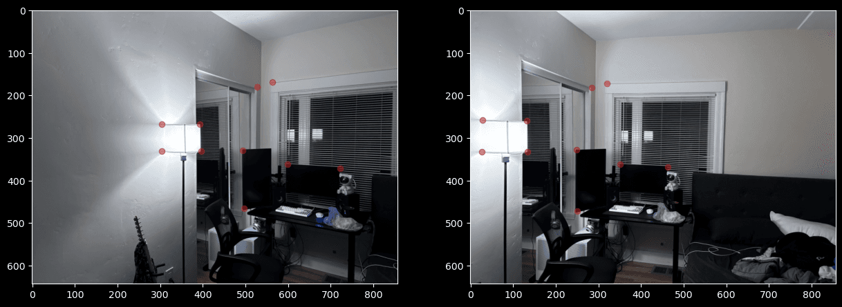
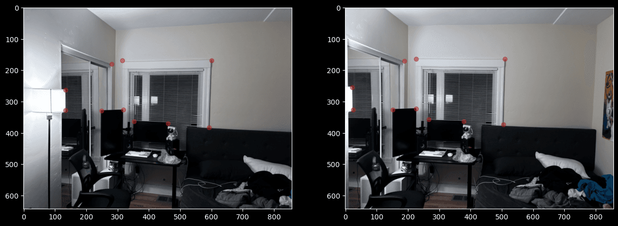
In order to get image with the same center of projection we can fix our camera at some point and only rotate it to get several images. We can then manually select correspondence points and use linear algebra to calculate homographies between different images. We select our correspondence points usually to be edges in corresponding pictures because they are easy to match. Below are pictures of corresponding points.
To calculate the necessary projective transformation we can solve a set of linear equations for the 8 parameters of the transformation. This means we need at least 4 points to compute this transformation. In practice it is helpful to use more than 4 points and solve the system using OLS. We derive out system of equations as shown below. Notice the scaling constant in projective transformation. For all of our purposes we can simply divide each component of the resulting 3D coordinate by the scaling constant to recover the homogenous output coordinate.
Image Rectification
Using the principles of projective transformations and homography we can rectify images, that is we can take an image of a rectangular object from a perspective where the image of the object is not rectangular and make it rectangular again. In order to do this we simply compute the homography between the corners of the object and four corners of a rectangle, then compute the transformation between the first set of points and the second. We then apply the transformation to the original image as shown below.
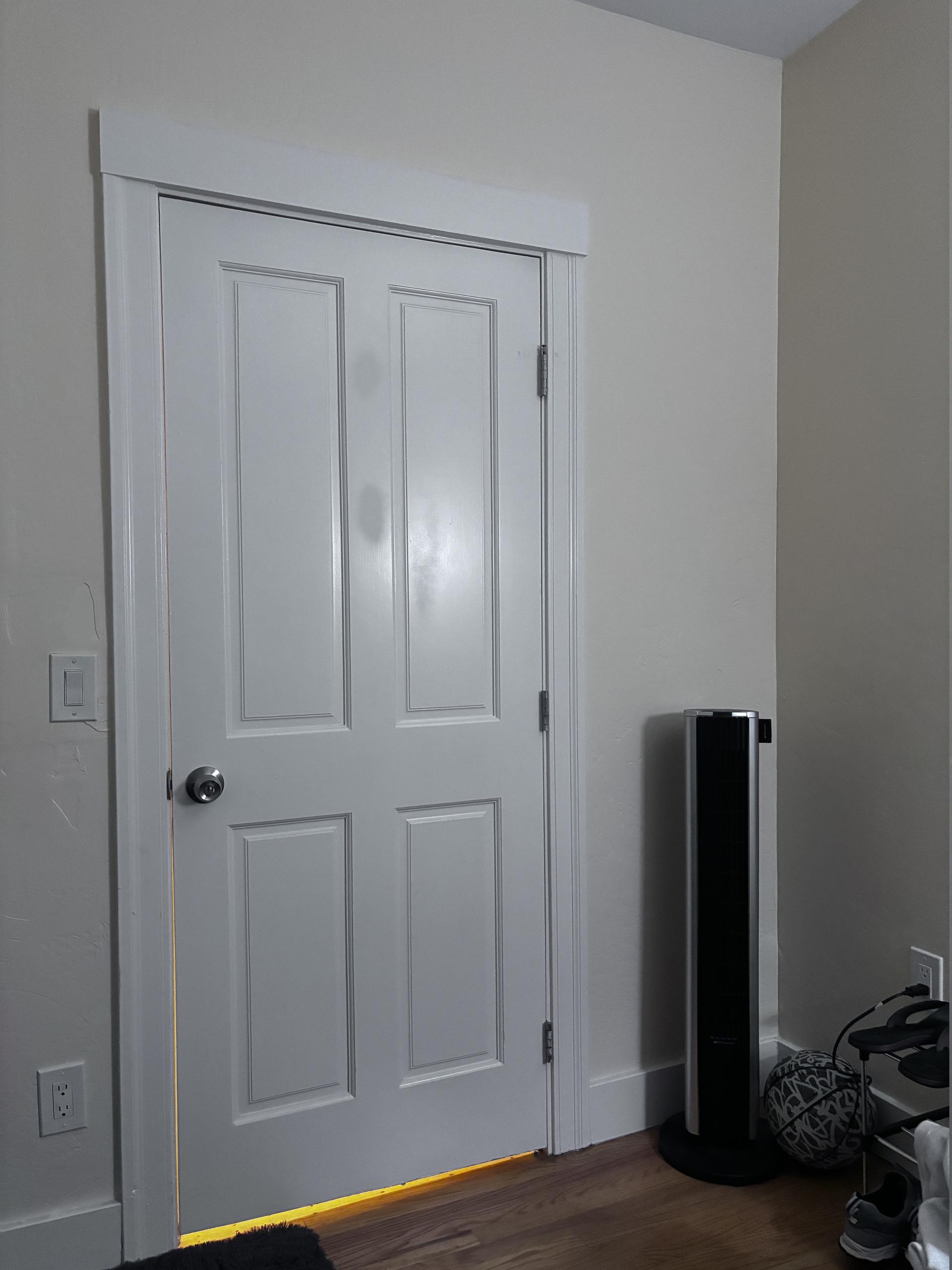
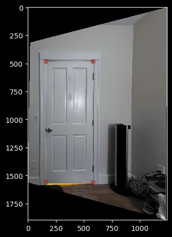
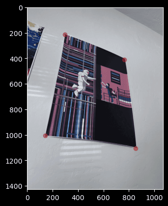
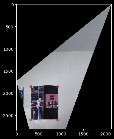
Image Stitching and Mosaics
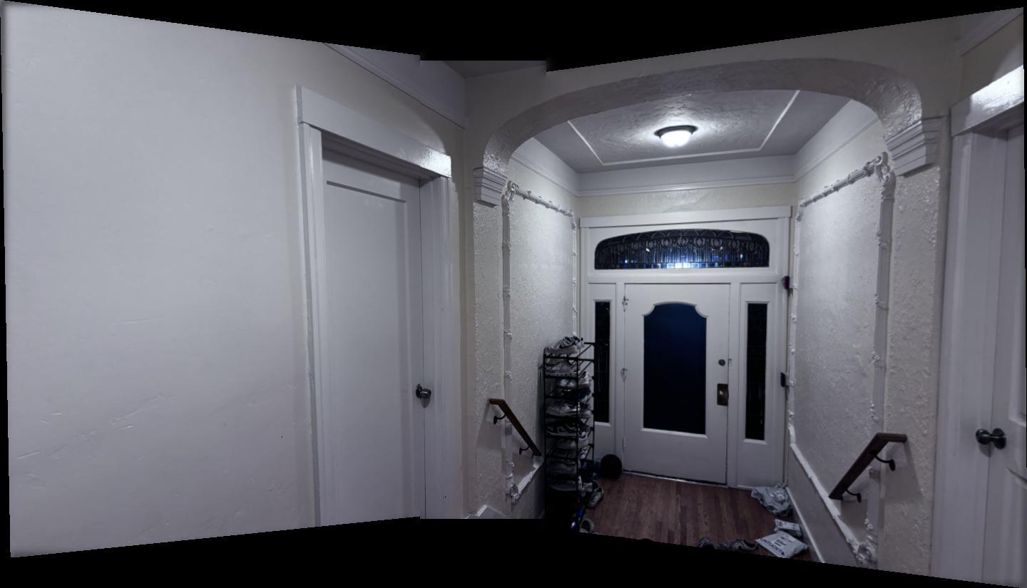
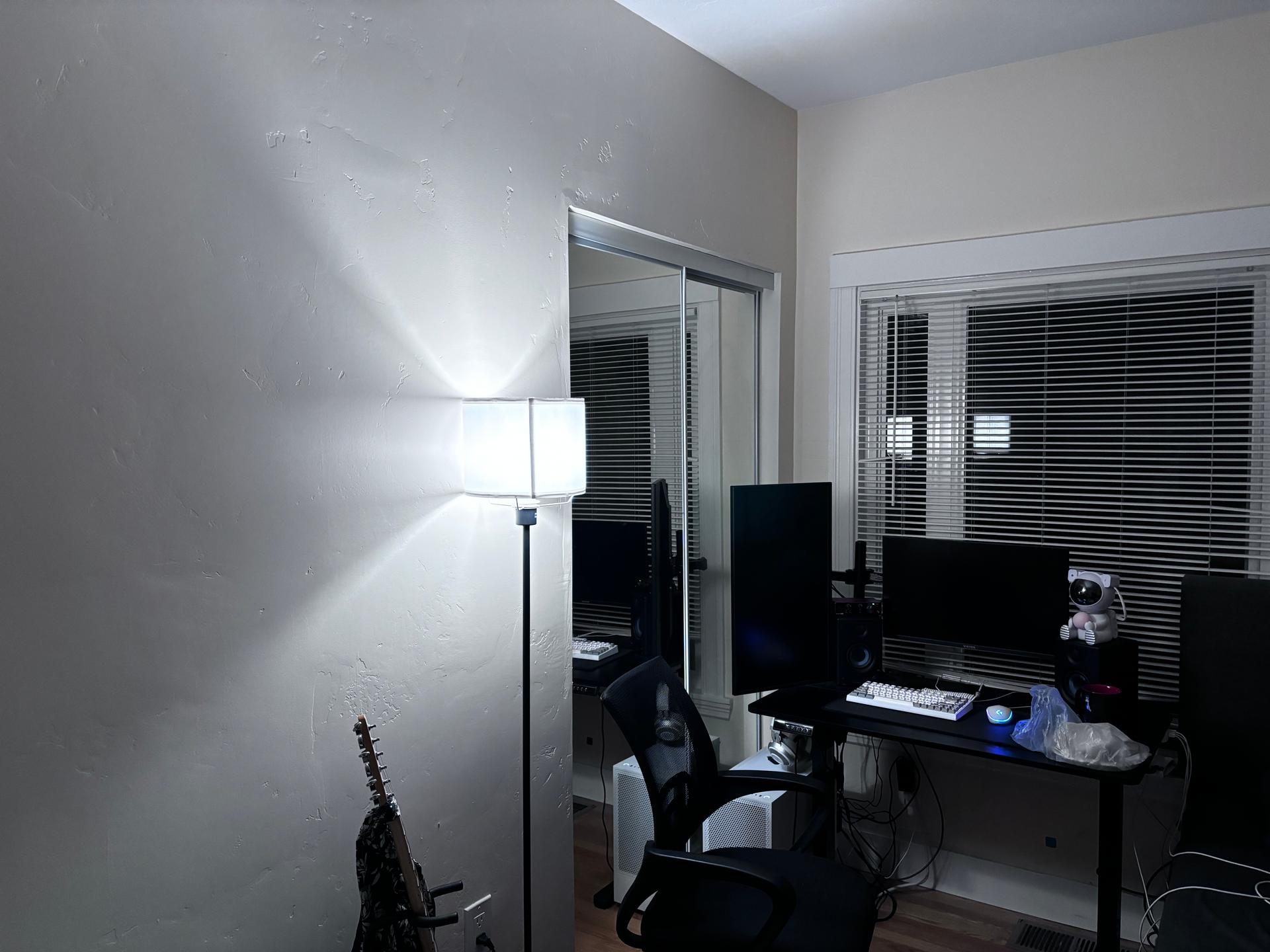
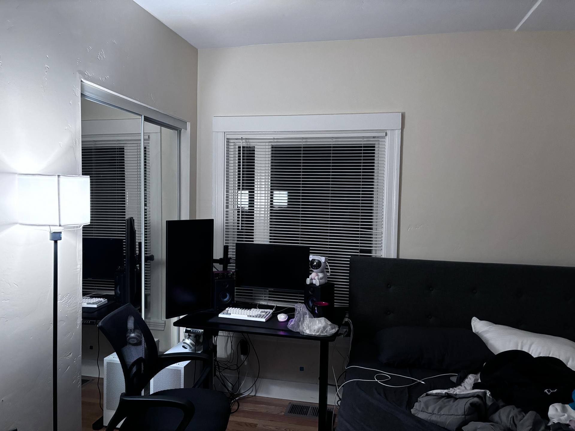
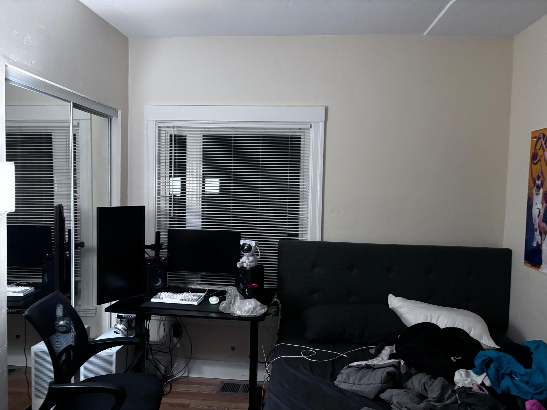
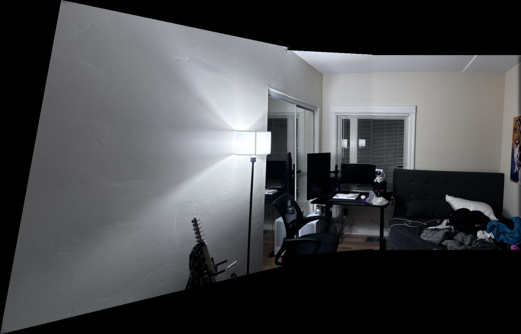
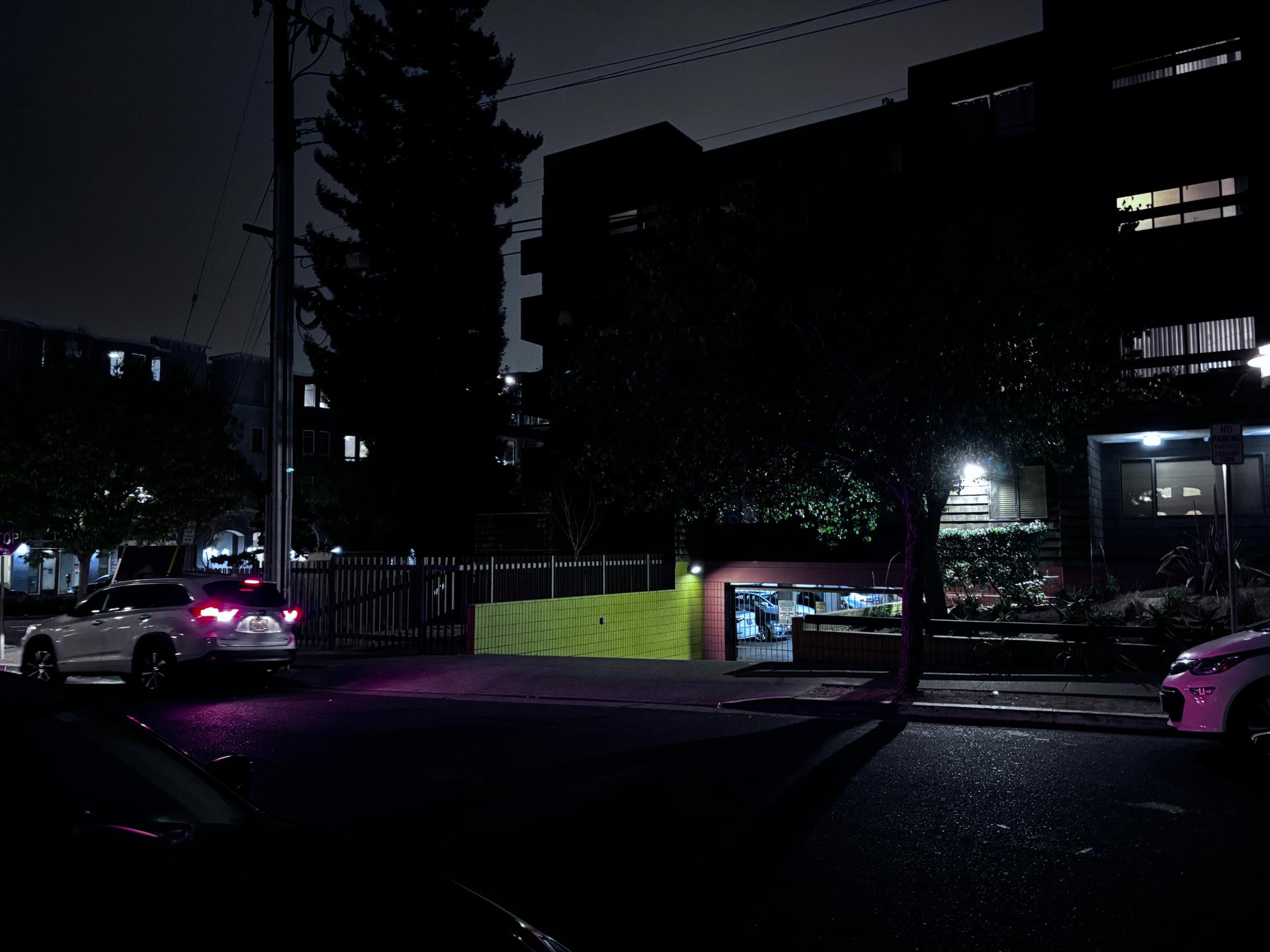
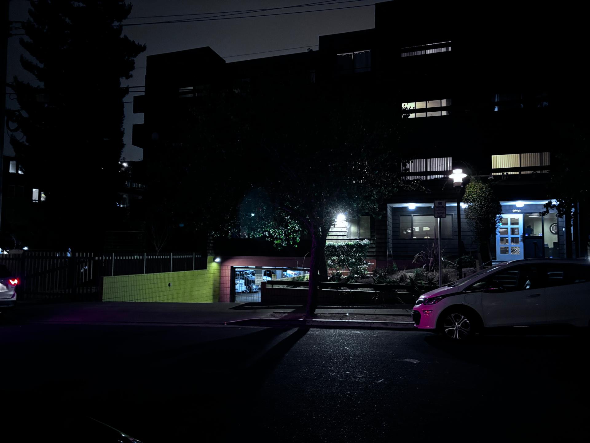
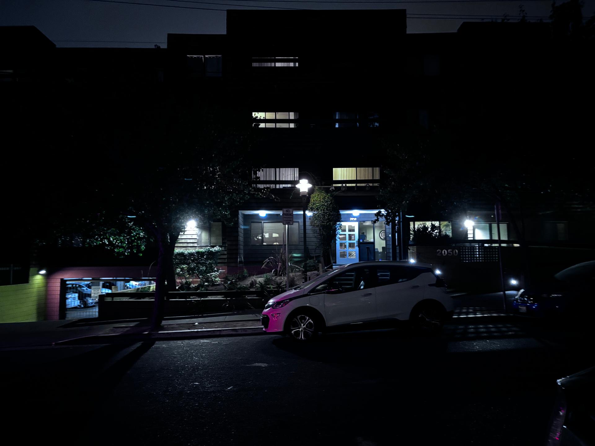
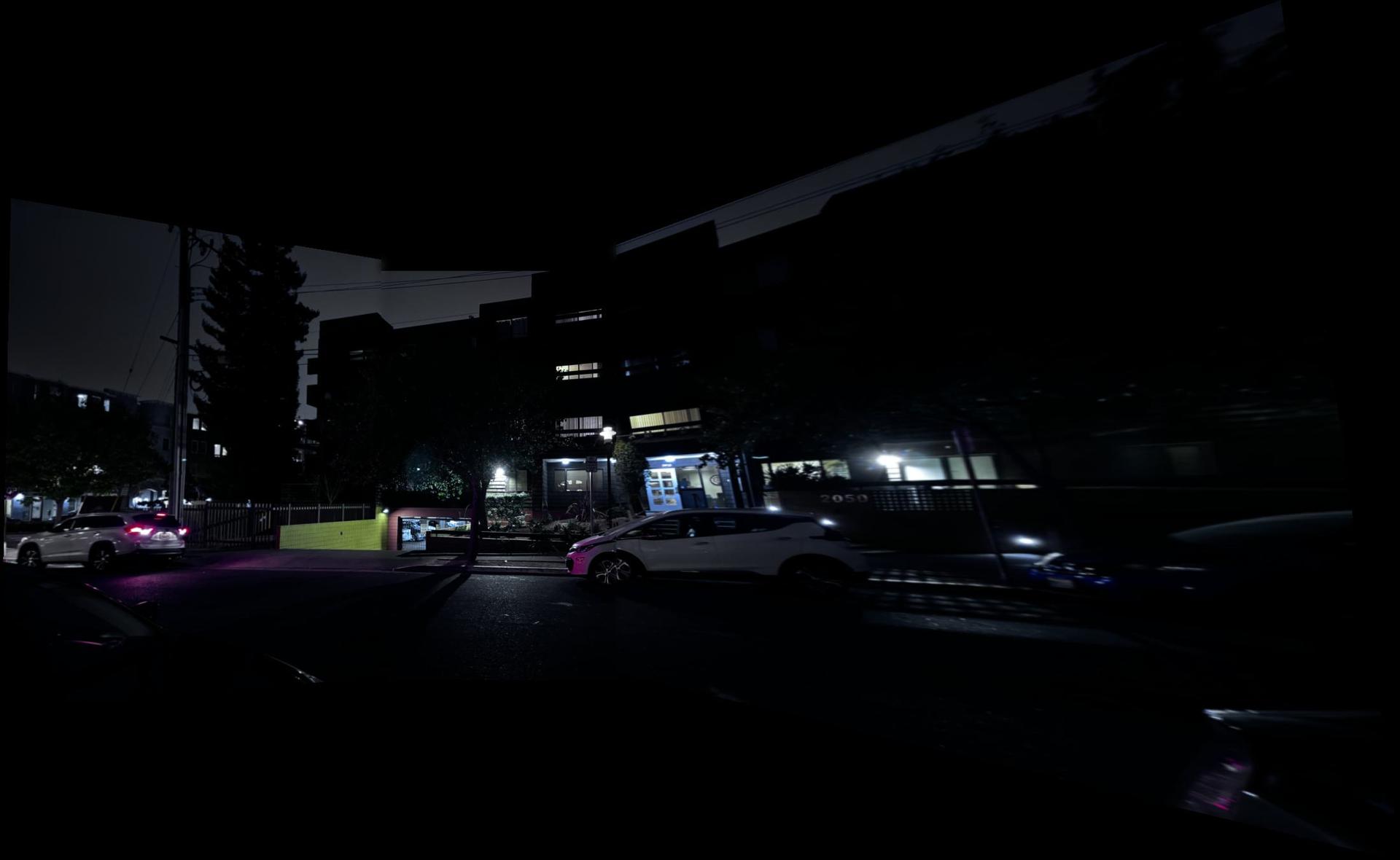
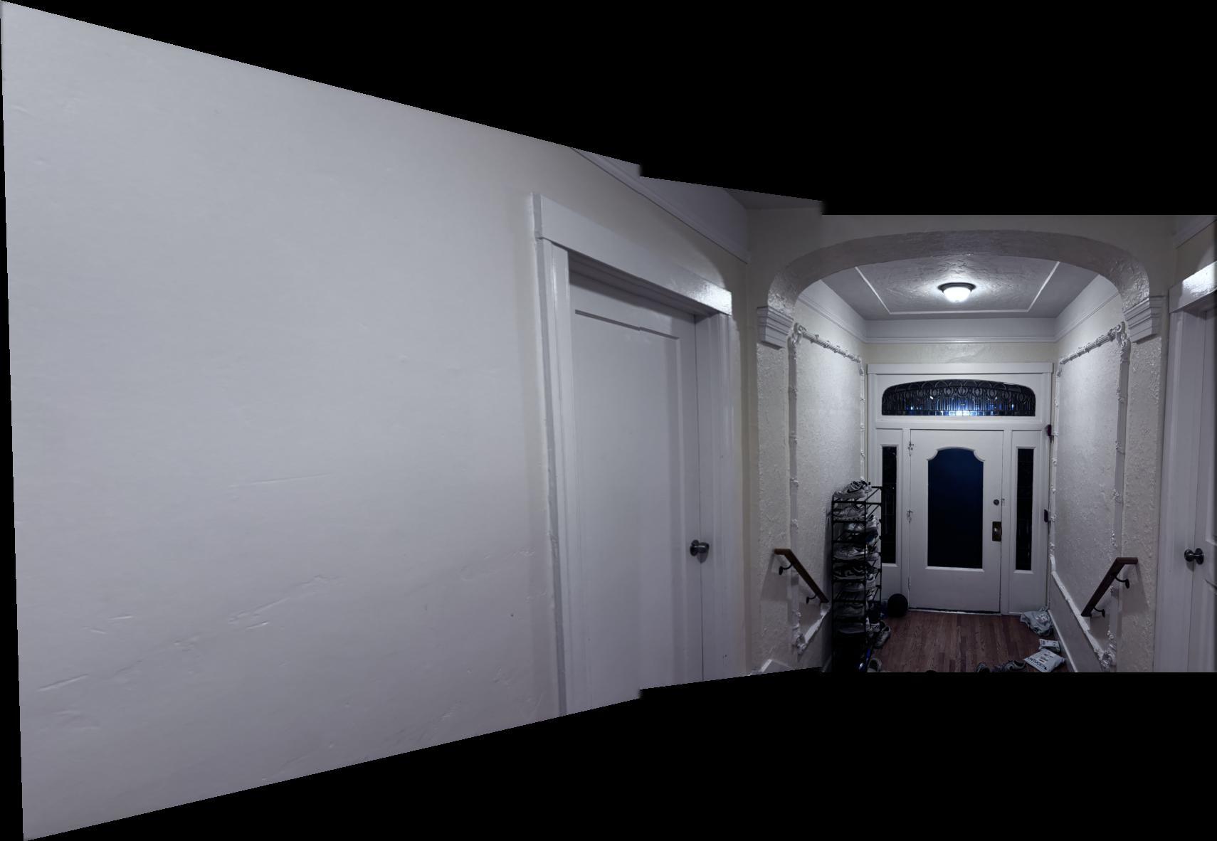
In order to stich our images together we can simply use the homographies we computed in the first section between our correspondence points to transform our images toward one image we choose. In this case we will use the center image as our central coordinate system. We can simply transform the images and then shift them the necessary amount as determined by our transformations output in order to align our images on the coordinate system. Once our images are aligned on a central coordinate system we can blend our images together to get our final result. For this project I used Laplacian stacks to blend my images which neatly deals with merging high frequency and low frequency components of both images. For more information check filtering project on the main page of my portfolio. Below are examples of images and their corresponding mosaics.
Detecting Points with Harris Corners
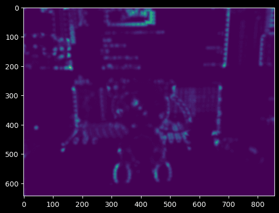
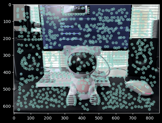
So far we have relied on manually selected feature points; however, this is time consuming and tedious. We will now automate this task through first detecting a large set of possible matching key-points and then selecting a subset of those points using several algorithms. Our first step will be to get a large set of possible key points. In order to do this we can use Harris Corners. Essentially the idea here is that good feature points often fall at corners because they are easy to match across images. In order to systematically find corners we can take the gradient in both the x and y dimensions, compute the second moment matrix, and analyze the diagonalized form of the matrix. If eigenvalues of the second moment matrix (M) are both larger and close to each other then we are likely at a corner because small changes in either of those directions would yield large changes in the image function. This can be formalized by calculating the corner response function det(M) / Trace(M). We can consider this functions local maximums as potential key-points. Shown below is an image, its corner response function plot, and the selected key-points.
Adaptive Non-Maximal Suppression
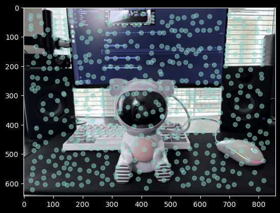
With our potential feature points we can now narrow our selection. This will improve the efficiency of our feature matching and outlier rejection in the next sections. We will use a technique known as Adaptive Non-Maximal Suppression in order to narrow our selection of points. This technique selects the points with the highest corner response while ensuring that points are reasonably spread out. It works by having a window and selecting the best point as measured by the corner response for that window. We then recursively reduce the size of the window and select the next best points until we get the number of specified points. For our purposes we selected 500 key-points using this method. In practice this set of points forms an ordered list which can be computed much more efficiently that the recursive approach. We compute this list and select the 500 best points to get the following result.
Feature Descriptors
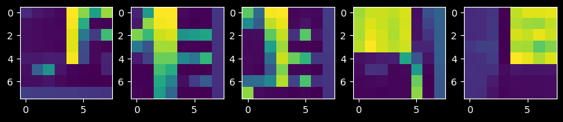
We now move towards the task of matching key-points across photos. Ideally across photos similar key points in regions of interest were found because in both images the corner response is high. We can take advantage of the fact to match the key points. In order to know if two points are similar we can look in a local region surrounding the point and compute a vector which says what the region looks like. We do this by sampling every 5 pixels in a 40x40 range surrounding the image to get an 8x8 sample which we flatten into a 64 dimensional vector as a feature descriptor. These vectors correspond to a specific key-point. Some of the pre-flattened feature descriptors are shown below.
Matching Key-Points
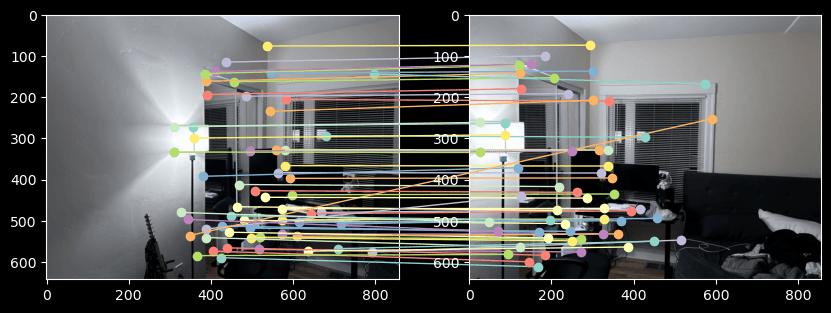
With our feature descriptors we can move on to the task of matching descriptors across images. Some properties that would be nice for our matches to have are symmetry (if x is a match to y, y is a match to x) and certainty (if x is a match to y1 then x is not close to being a match to y2). A natural approach to finding pairs of matching feature detectors is to use nearest neighbors where we compute the Euclidean distance between feature detectors and choose the first neighbor of each descriptor to be its pair. To get symmetry as desired we can ensure that features x and y are only a pair if x is the first neighbor of y and y is the first neighbor of x. This will ensure that if y is the first neighbor of x1 and x2 then only one of the pairs matches with y. In order to get the second desired property we can consider the 2nd neighbor of each feature point. Ideally the distance from a points first neighbor should be much less than the distance to the points second neighbor. This will ensure that certainty is preserved. We can simply compute the ratio of these two distances and threshold at a chosen hyper-parameter value in order to get this property. After completing these steps we get the following result.
Outlier Rejection with RANSAC
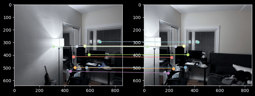
We can see that many of our feature matches are decent; however, there are still some serious outliers that will hinder our mosaic if we were to try and compute our homographies with these points. These points are particularly difficult to handle due to the nature of their being. These points survived all of our other attempts to remove outliers and find correct points. In order to solve this we turn to RANSAC. RANSAC is an exponential runtime algorithm in the number of parameters, but it can be very precise in removing outliers. With so few points left the exponential runtime will not prove to be a hinderance, and we will still be able to remove outliers in reasonable time. RANSAC essentially picks a random combination of points and computes the desired transformation for those points. It then uses that transformation on every point pair and computes how many of the point pairs agreed with that transformation (for a point pair x and y we want T(x) to be sufficiently close to y as determined by a hyper-parameter). We compute the total number of pairs which agreed with the transformation and compare it to the previous best total number of pairs. If the total number of pairs for this transformation is larger we set it as our best and remember the set of points which agreed with the transformation. We repeat this process for some N number of iterations. If the algorithm is run for enough iterations we will eventually find a set of points which are free of outliers that we can use to compute our homography.
Auto-Generating Mosaics
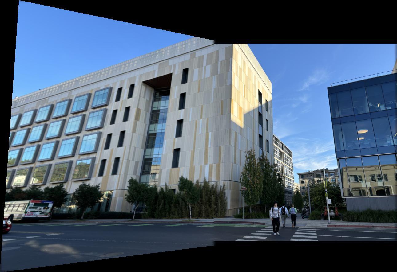
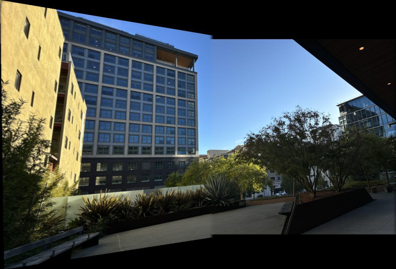
With our automatically selected feature points in each image we are now ready to combine everything to automatically compute mosaics. We simply follow the following steps: detect features using Harris corners, narrow the selection using ANMS, get feature descriptors using MOPS, find matching feature descriptors, remove outliers with RANSAC, compute homographies, warp images into some base image, and finally blend the images together to get our mosaic. Here are some of the following results from running this process.
Conclusion
The first three projects all come together in the first part of this project. We use pyramids, blurring, and warping to get our image mosaics. We then introduced concepts from optimization such as searching for local maximums and the second moment matrix to automatically find correspondence points. We finish by using RANSAC and combining everything to get our final results.